Training Energy-Based Models

Training Methods of Energy Based Models

Energy based models try to learn unnormalized probabilities or energies of a input based on the given data distribution. The functions assign lower energies to the input data while assigning higher energies to unseen data during training. Let this energy function be parameterized by parameters $\theta$, hence, energy for a random variable $x$ is given by $E_\theta(x)$. But this energy itself means nothing until we can convert it to a probability, which, we can do by using the simple probability formula, that the probability of the event is the occurance of the event divided by the occurance of all the other events, i.e.,

p_\theta(x) = \frac{exp(-E_\theta(x))}{\int_{x} exp(-E_{\theta}(x))dx }

Let us define the integral as a constant,

\int_x \exp(-E_{\theta}(x))dx = Z_{\theta}

this new constant, $Z_\theta$, is called the normalizing constant or the partition function, such that $\int p_\theta(\mathbf{x}) \mathrm{d} \mathbf{x}=1$. This constant is usually intractable, why so? Because as you can see the calculation of this constant requires calculating the integral over all the possible values of the random variable $x$. This is what usually makes training energy based models difficult, however, there are quite a few methods to approximate the density function which can make the learning a bit more efficient.

Our goal is to train the get the parameters $\theta$ for the EBM such that it models the true data distribution, which essentially as in most machine learning boils down to Maximum Likelihood Estimation. The MLE can be defined as,

\theta^* = argmax \space \mathbb{E}_{x\sim p_{data}}[\log(p_{\theta}(x))]

As mentioned mentioned above computing the $p_\theta$ in the above objective is infeasible.

Since, we have our objective defined to calculate $\theta^*$, we need to compute the gradient of the log-likelihood, which breaks down to

\nabla_{\boldsymbol{\theta}} \log p_\theta(\mathbf{x})=-\nabla_{\boldsymbol{\theta}} E_{\boldsymbol{\theta}}(\mathbf{x})-\nabla_{\boldsymbol{\theta}} \log Z_{\boldsymbol{\theta}} .

The first term can be calculated easily using automatic differentiation tools. The second term is tricky, but it turns out we can express this as an expectation:

\nabla_{\boldsymbol{\theta}} \log Z_{\theta}=\mathbb{E}_{\mathbf{x} \sim p_\theta(\mathbf{x})}\left[-\nabla_\theta E_\theta(\mathbf{x})\right]

This means if we can sample from our model $p_{\theta}(x)$, we can estimate this gradient term!

Markov Chain Monte Carlo (MCMC)

MCMC methods are probably one of the most infamous methods in engineering and science in general. These methods allows us to draw samples from complex distributions like EBM without exactly knowing the distribution. How does it do it?

Start: Begin at a random point in the distribution
Wander: Move around the distribution following specific rules (e.g. Langevin dynamics).
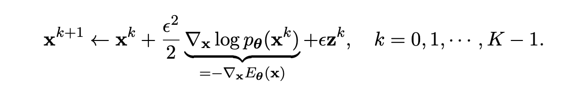
Sample: Periodically record the current position as a sample. There are many algorithms that provide us these rules to move around, one of the popular methods is Langevin MCMC. At first, we draw a random sample from a simple prior distribution (usually Gaussian noise) and then iteratively denoise this using Langevin dynamics with a step size $\epsilon > 0$ (we also some stochasticity $z^k$ at each step to help preserve the multimodality),

This whole training process can be written in these two python functions,

def langevin_dynamics(model, x, num_steps=100, step_size=0.1):
    x.requires_grad_(True)
    for _ in range(num_steps):
        energy = model(x)
        grad = torch.autograd.grad(energy.sum(), x)[0]
        x = x - step_size * grad + np.sqrt(2 * step_size) * torch.randn_like(x)
    return x.detach()

def train_ebm(model, data, num_epochs=500, batch_size=100, lr=1e-4):
    optimizer = optim.Adam(model.parameters(), lr=lr)
    
    for epoch in range(num_epochs):
        for i in range(0, len(data), batch_size):
            real_samples = data[i:i+batch_size]
            fake_samples = torch.randn_like(real_samples)
            fake_samples = langevin_dynamics(model, fake_samples)
            
            real_energy = model(real_samples)
            fake_energy = model(fake_samples)
            
            loss = real_energy.mean() - fake_energy.mean()
            
            optimizer.zero_grad()
            loss.backward()
            optimizer.step()
        
        if (epoch + 1) % 100 == 0:
            print(f"Epoch [{epoch+1}/{num_epochs}], Loss: {loss.item():.4f}")

Score Based Matching

While MCMC methods offer a powerful approach to training Energy-Based Models, they can sometimes be computationally expensive and face challenges with mixing and convergence, especially in high-dimensional spaces. Score Matching is an alternative method that circumvents some of these issues by focusing on a different aspect of the model: its score function. The score function is a fundamental concept in statistics that provides a different perspective on probability distributions. For a probability density function p(x), the score function is defined as the gradient of the log-probability with respect to the input, $\nabla_x \log(p(x))$. In the context of EBMs, as mentioned previously this takes an elegant form

\nabla_{\mathbf{x}} \log p_\theta(\mathbf{x})=-\nabla_{\mathbf{x}} E_{\boldsymbol{\theta}}(\mathbf{x})-\underbrace{\nabla_{\mathbf{x}} \log Z_\theta}_{=0}=-\nabla_{\mathbf{x}} E_\theta(\mathbf{x}) .

This simple relationship allows us to work directly with the energy function $E(x)$ without worrying about the intractable normalization constant that often complicates MCMC-based training.

Fisher Divergence: To train our EBM using score matching, we need a way to measure how well our model’s score function matches that of the true data distribution. This is where the Fisher divergence comes into play. The Fisher divergence between two distributions p and q is defined as:

D_F\left(p_{\text {data }}(\mathbf{x}) \| p_{\boldsymbol{\theta}}(\mathbf{x})\right)=\mathbb{E}_{p_{\text {data }}(\mathbf{x})}\left[\frac{1}{2}\left\|\nabla_{\mathbf{x}} \log p_{\text {data }}(\mathbf{x})-\nabla_{\mathbf{x}} \log p_{\boldsymbol{\theta}}(\mathbf{x})\right\|^2\right]

In other words, it measures the expected squared difference between the score functions of p and q. By minimizing this divergence, we can train our EBM to closely match the true data distribution.

If we have access to true pdf, then we can calculate the energy model directly by minimizing this divergence

def log_true_pdf(x):
    dist1 = torch.distributions.MultivariateNormal(torch.tensor([-2., -2.]), torch.eye(2)*0.5)
    dist2 = torch.distributions.MultivariateNormal(torch.tensor([2., 2.]),  torch.eye(2)*0.5)
    return torch.log(0.5 * torch.exp(dist1.log_prob(x)) + 
                      0.5 * torch.exp(dist2.log_prob(x)))

def fisher_divergence(model, x):
    x.requires_grad_(True)
    energy = model(x)
    model_score = -torch.autograd.grad(energy.sum(), x, create_graph=True)[0]

    x_detached = x.detach().requires_grad_(True)
    true_score = -torch.autograd.grad(log_true_pdf(x_detached).sum(), x_detached, create_graph=True)[0]

    fisher_div = 0.5 * torch.mean((model_score - true_score)**2)
    return fisher_div

def train_energy_model(model, data, epochs=1000, lr=0.00001, batch_size=128):
    optimizer = optim.Adam(model.parameters(), lr=lr)
    data_loader = torch.utils.data.DataLoader(data, batch_size=batch_size, shuffle=True)

    for epoch in range(epochs):
        for batch_idx, batch_data in enumerate(data_loader):
            optimizer.zero_grad()
            loss = fisher_divergence(model, batch_data)
            loss.backward()
            optimizer.step()

        if epoch % 100 == 0:
            print(f'Epoch {epoch}, Loss: {loss.item()}')

Denoising Score Matching

Well, in most of the situation we do not have access to this log_true_pdf function, in such cases, Denoising Score Matching provides an elegant solution. The core idea of DSM is to work with a noise-perturbed version of our data, which allows us to sidestep the need for knowing the true data distribution while also making the method more robust to discrete or sharp features in the data.

The process begins by adding noise to our original data points. Typically, we use Gaussian noise, which has some desirable mathematical properties. This noise addition serves two purposes: it smooths out the data distribution, making it easier to model, and it provides us with a known reference point for our optimization process.

Once we have our perturbed data, we pass it through our energy model. The energy model, at its core, is trying to capture the structure of our data distribution. By computing the energy of the perturbed data points, we’re asking our model to make sense of this smoothed version of our data landscape.

The next crucial step is computing the score of our model for these perturbed data points. Recall that the score is the negative gradient of the log-density, which in the case of an EBM, simplifies to the negative gradient of the energy function. This score represents our model’s belief about the local structure of the data distribution at each point.

Now comes the key insight of DSM: for Gaussian noise, we know the optimal denoising direction analytically. It’s simply the noise vector scaled by the inverse of the noise variance. This known quantity serves as our target, or “ground truth,” in the optimization process.

The DSM loss is then computed as the mean squared difference between our model’s score and this optimal denoising direction. By minimizing this loss, we’re effectively training our model to denoise the perturbed data points optimally. This process, somewhat surprisingly, is equivalent to minimizing the Fisher divergence between our model and the noise-perturbed data distribution.

Noise Contrastive Estimation

The main idea behind Noise Contrastive Estimation (NCE) is to distinguish data distribution from noise distribution. Imagine we have a set of genuine data points ${x_1,x_2,…,x_n}$ sampled from the true data distribution $p_{\text{data}}$, and a set of noise points ${y_1, y_2, \ldots, y_m}$ sampled from a known noise distribution $p_{\text{noise}}$. The idea behind NCE is to teach the model to differentiate between these real data points and the noise points. Instead of directly estimating the probability distribution of the data, NCE focuses on the task of classification, which is more straightforward.

The key to NCE lies in the computation of energy values for both data and noise samples using energy-based model. This energy model assigns a score to each sample, where lower energy corresponds to high likelihood. We aim to train the model such that real data points ahve lower energy score compared to noise points.

Mathematically, for a given sample $x$ from the data and $y$ from the noise, our energy model $E_{\theta}$(.) computes the energy value $E_{\theta}(x)$ and $E_{\theta}(y)$. To differentiate betweeen data and noise, we calculate the log-odds for each type of sample. The log-odds for a data sample $x$ can be expressed as:

\log \frac{p_{\text {dstat }}(x)}{p_{\text {moles }}(x)}=-E(x)-\log k

where $k$ is the noise ratio (the ratio of noise samples to data samples). Similarly, for a noise sample $y$, the log-odds are

\log \frac{p_{\text {data }}(y)}{p_{\text {mulef }}(y)}=-E(y)+\log k

(If you have ever used particle filter in robotics for mapping, this might look similar to you. The real datapoints here are obstacles and other points are free space, we aim to get the probability distribution of the obstacle over the space.)

The training objective is to maximize the likelihood of correctly classifying the samples. This is achieved by minimizing the binary cross-entropy loss, which is a standard loss function for classification tasks. For data samples, the target label is 1 (data), and for noise samples, the target label is 0 (noise).

def nce_loss(energy_model, data, noise, noise_ratio=1):
    batch_size = data.shape[0]
    
    # Concatenate data and noise
    all_samples = torch.cat([data, noise], dim=0)
    
    # Compute energy for all samples
    energies = energy_model(all_samples).squeeze()
    
    # Split energies for data and noise
    data_energies = energies[:batch_size]
    noise_energies = energies[batch_size:]
    
    # Compute log-odds
    log_odds_data = -data_energies - torch.log(torch.tensor(noise_ratio, dtype=torch.float32))
    log_odds_noise = -noise_energies + torch.log(torch.tensor(noise_ratio, dtype=torch.float32))
    
    # Compute binary cross-entropy loss
    loss_data = nn.functional.binary_cross_entropy_with_logits(log_odds_data, torch.ones_like(log_odds_data))
    loss_noise = nn.functional.binary_cross_entropy_with_logits(log_odds_noise, torch.zeros_like(log_odds_noise))
    
    # Combine losses
    loss = loss_data + noise_ratio * loss_noise
    
    return loss

def train_nce(energy_model, num_epochs=1000, batch_size=128, noise_ratio=1, lr=0.001):
    optimizer = optim.Adam(energy_model.parameters(), lr=lr)
    
    for epoch in range(num_epochs):
        # Sample data and noise
        data_batch = sample_data(batch_size)
        noise_batch = sample_noise(batch_size * noise_ratio)
        
        # Compute loss
        loss = nce_loss(energy_model, data_batch, noise_batch, noise_ratio)
        
        # Backpropagation and optimization
        optimizer.zero_grad()
        loss.backward()
        optimizer.step()
        
        if (epoch + 1) % 100 == 0:
            print(f"Epoch {epoch+1}/{num_epochs}, Loss: {loss.item():.4f}")

References

“How to Train Your Energy-Based Models”, Yang Song, Diederik P. Kingma, 2021, arxiv.org/abs/2101.03288