Memorization vs Generalization

Memorization and generalization are two concepts in machine learning that have personally confused me for a long time. After sitting through countless seminars from guest faculty and PhD students, I often found myself even more puzzled: When is memorization good? When is it bad? And perhaps most importantly - what exactly are memorization and generalization?

It turns out the answer isn’t simple and depends heavily on context. If your task requires recalling training data, then memorizing that data precisely might actually help with test performance. However, if your task involves generalizing to unseen examples that can only be understood by learning the true underlying data-generating process, then exact memorization might hurt - this is what we typically call overfitting.

But there’s one thing that’s often overlooked: Sometimes memorization is actually necessary for optimal generalization, particularly when dealing with real-world data distributions. In this post, I’ll focus on how the structure of data distributions can affect memorization and why it might be optimal for models to memorize certain examples.

Memorization

While we mostly think about memorization informally, having a precise definition helps clarify our discussion. Following Feldman et al., we can define memorization in terms of how much a single training example influences the model’s prediction on that same example.

Formally, for a dataset S = ((x₁,y₁),…,(xₙ,yₙ)) and a learning algorithm A, the memorization score for example $i$ is:

mem(A, S, i) = Pr[A(S) predicts yᵢ on xᵢ] - Pr[A(S\i) predicts yᵢ on xᵢ]

where S\i is the dataset S with example i removed. In other words, we measure how much more likely the model is to predict the correct label when it has seen the example versus when it hasn’t.

This definition captures our intuitive notion of memorization - if the model can only predict correctly on an example when it has seen that exact example during training, we say it has memorized that example. The memorization score will be high (close to 1) in such cases.

Generalization:

Generalization is a very messy topic, there are many types of generalization one-shot, few-shot, cross-domain, in-distribution, out-of-distribution etc., But here let us consider that we are interested in in-distribution generalization, i.e., there is no distribution shift between training set and test-set. A useful metric in such a case is Generalization gap. Simply put, it’s the difference between how well a model performs on its training data versus on new, unseen test data. More formally,

Generalization Gap = Training Error - Test Error

You need to memorize to generalize

Now that we have defined the defnitions of memorization and generalization, let us move on to consider their relationship and how it can be counterintuitive at first but gets more clear as we understand their interplay. For the rest of the post, I will be mostly discussing the results from Feldman (2020).

If you squint enough, most of the real world data will look like this. This is called Zipf’s distribution (or law), is a specific instance of Power law where the exponent is typically very near to -1. It is a natural property of Data generated by time-dependent rank-based systems (Fernholz & Fernholz, 2020). Originally, it was coined in linguistics (Zipf, 1935), however, it is quite universal. As an aside, here is also an interesting video on the natural occurence of zipf’s law.

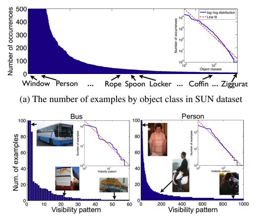
As seen, if you just take the class labels or the subpopulations within a class label they roughly follow the Zipf distribution. This means the frequency at which different patterns occur in our data follows a predictable but highly skewed pattern - a few examples appear very frequently, while the majority of examples are relatively rare.

The main result from Feldman’s paper is a theorem that formalizes when and why memorization can be necessary. Before diving into the math, let’s understand what it’s trying to show.

Imagine we’re training a model on a dataset where some patterns appear frequently while others are rare (like our Zipf distribution). The theorem tells us two key things:

1. How much error we’ll get if we don’t memorize certain examples
2. How this error depends on how frequently similar examples appear in our data

Here’s the formal statement:

Theorem 2.3. Let $\pi$ be a frequency prior with a corresponding marginal frequency distribution $\bar{\pi}^N$, and \(\mathit{F}\) be a distribution over $Y$. Then for every learning algorithm $\mathit{A}$ and every dataset $Z \in(X \times Y)^n$ : \(\overline{\operatorname{err}}(\pi, \mathit{F}, \mathit{A} \mid Z) \geq \operatorname{opt}(\pi, \mathit{F} \mid Z)+\sum_{\ell \in[n]} \tau_{\ell} \cdot \operatorname{errn}_Z(\mathit{A}, \ell)\)

where

In particular,

Let’s break this down piece by piece:

• The left side $\overline{\operatorname{err}}(\pi, \mathit{F}, \mathit{A})$ represents how well our learning algorithm A performs
• $\operatorname{opt}(\pi, \mathit{F})$ is the best possible performance any algorithm could achieve
• The sum term $\sum_{\ell \in[n]} \tau_{\ell} \cdot \operatorname{errn}_S(\mathit{A}, \ell)$ is the key insight - it’s the extra error we get for not fitting (memorizing) training examples

The most interesting part is $\tau_{\ell}$, which measures the “cost” of not memorizing examples that appear ℓ times in our dataset. For examples that appear only once ($\ell=1$), this cost becomes substantial when:

1. The data follows a long-tailed distribution (like Zipf’s law)
2. There are many examples with frequency around 1/n
3. Our dataset size n is large

The main takeaway of this result is that any learning algorithm that fails to fit (or memorize) examples in the training data will incur additional error beyond what’s theoretically optimal.

Seeing it Work in Practice

The theory sounds compelling, but how do we actually verify it? How can we see this memorization happening in real neural networks and - more importantly - prove that it’s helping? A follow-up work by Feldman and Zhang (2020) tackles exactly these questions.

Measuring Memorization in Practice

Remember our formal definition of memorization that looks at how predictions change when we remove examples? While mathematically elegant, it’s completely impractical - we’d need to retrain our model thousands of times for each training example! Instead, the authors developed a clever approximation:

1. Train multiple models (say 2000) on random subsets of the training data
2. For each example, compare how well models predict it when it’s in their training set versus when it’s not
3. This gives us an estimate of the memorization score without needing to retrain from scratch for each example

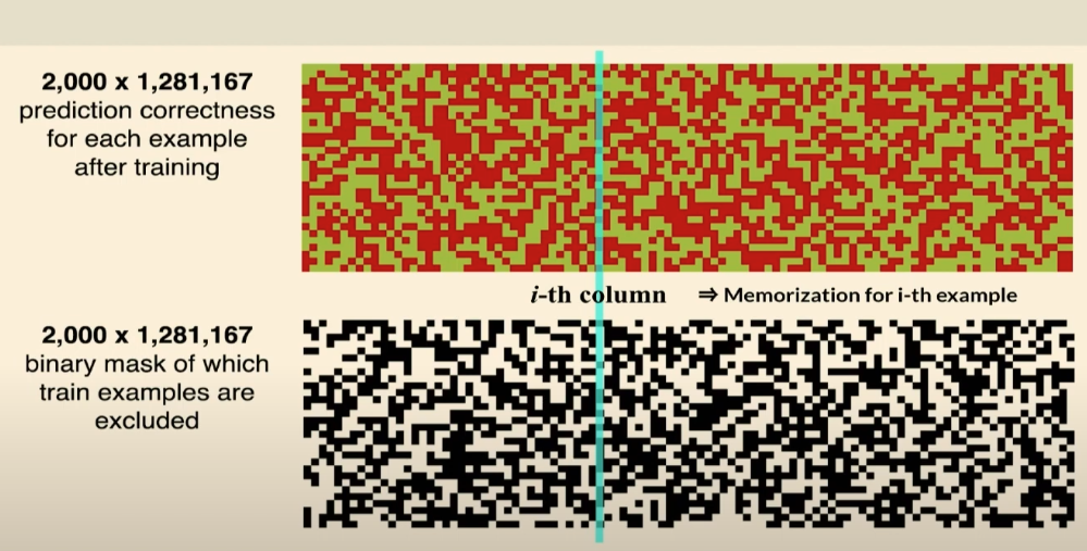
In this visualization, each row represents one model, each column is a training example, and:

• The top shows prediction accuracy (brighter = more accurate)
• The bottom shows which examples were used to train each model (white = used, black = not used)
• Looking at any column tells us how well models do on that example when they’ve seen it versus when they haven’t

What Gets Memorized?

When applying this to real datasets like CIFAR-100 and ImageNet, the results align remarkably well with the theory. On ImageNet:

• About 32% of training examples show high memorization scores (≥0.3)
• These aren’t random examples - they’re a mix of:
  • Outliers and potentially mislabeled examples
  • Most importantly, atypical but valid examples that represent rare subpopulations

Proving Memorization Helps

The real test comes when we remove these memorized examples. The authors found:

1. Removing the most memorized 32% of examples hurts accuracy by 3.4%
2. Removing the same number of random examples only causes a 2.6% drop
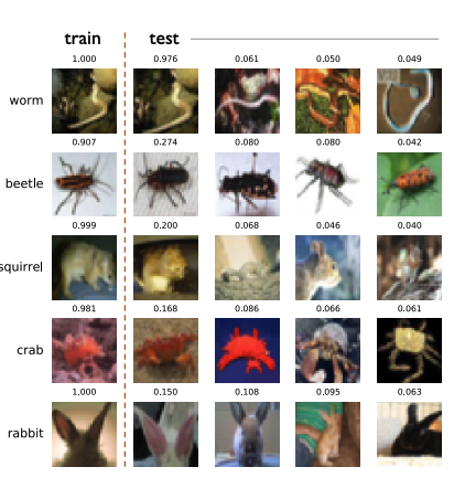
3. Most crucially, they found pairs of training and test examples where:
   • The training example was memorized
   • That specific training example significantly helped predict a similar test example
   • The test example wasn’t helped much by other training examples

This last point is exactly what we’d expect from the theory - these are likely examples of rare subpopulations where we only have one or two training examples to learn from!

What’s also interesting is that most test examples that benefit from memorization are helped by exactly one training example. In ImageNet, out of 1,462 test examples showing significant influence from memorized training examples, 1,298 were influenced by just one training example. This is exactly what we’d expect if these examples represent rare subpopulations in the long tail of our data distribution!

We can’t just throw out “outliers” or examples that seem to require memorization - they might be our only examples of important rare cases, there is no way to distinguish between genuinely rare example and an outlier, atleast that I know of. This is especially crucial when dealing with datasets that naturally have long tails, which is basically any real-world data. Similarly, when we try to make our models smaller or more private (which inherently limits their ability to memorize), we need to be aware that we might be disproportionately hurting performance on rare cases. This could create serious fairness issues if these rare cases correspond to minority groups or important edge cases.

The data even tells us something interesting about how neural networks accomplish this memorization. It turns out most of the memorization happens deep in the network’s representations, not just in the final layer. When the authors tried to replicate these effects by only training the final layer while keeping earlier representations fixed, the memorization patterns completely disappeared.

So what does all this mean for the apparent contradiction between memorization and generalization? In many real-world scenarios, memorization isn’t the enemy of generalization - it’s necessary for it. When our data has a long tail (and it almost always does), being able to memorize rare examples is crucial for achieving optimal performance across everything we care about.

Other Works

Grokking: From Memorization to True Understanding Grokking, although the name is trendy, represents a classical phenomenon where regularized models transition from memorization to generalization. It fundamentally connects to Occam’s razor principle (or minimum description length) that favors the simplest explanation. While recent work by DeMoss et al., has explored these transitions in controlled settings like modular arithmetic, we still lack understanding of how these patterns manifest in natural distributions. Studying grokking in the context of long-tailed distributions could provide valuable insights into how models progress from memorization to true generalization.

Data Pruning Data pruning helps us understand which examples we can remove while maintaining test performance. Paul et al., (2023) proposed the Gradient Normed (GraNd) and Error L2-Norm (EL2N) scores to identify important training examples. Interestingly, these scores don’t correlate with memorization scores, suggesting they capture different aspects of example importance. The samples that models consider “hard” may not be the same as those underrepresented in the population. This opens up interesting directions for connecting memorization scores, sample hardness, and learning dynamics.

Active Learning: Optimizing Data Collection Active learning becomes particularly relevant as we approach the limits of scaling with current datasets. The key question shifts from how to learn from existing data to where we should focus our data collection efforts. While traditional methods based on uncertainty are well-studied, approaches based on training dynamics, as explored by Kang et al., (2024), could offer new insights. Understanding memorization patterns could help identify underrepresented subpopulations and guide efficient data collection strategies. This connects directly back to our discussion of long-tailed distributions - we might want to deliberately oversample rare but important cases to improve model performance on crucial edge cases.