Per Sample Gradients

Per sample gradients are cool. They can be used for many things, such as data-attribution, curriculum learning, multi-task learning, and scaling. However, Pytorch provides only batch gradients with no way to compute per-sample gradients. You can still use libraries like Opacus to get the per-sample gradients, I thought it will be interesting to write it down so that it will be helpful to understand how to efficiently calculate the per-sample gradients.

What are Per-Sample Gradients and How they are helpful?

Let $\mathit{X}$ be our input space and $\mathit{Y}$ be our output space. For a dataset $\mathit{D} = {(x_i, y_i)}_{i=1}^n$ where $x_i \in \mathit{X}$ and $y_i \in \mathit{Y}$, a neural network can be viewed as a parameterized function $f_\theta: \mathit{X} \rightarrow \mathit{Y}$ with parameters $\theta \in \Theta$. For each sample $(x_i, y_i)$, we define a loss $\ell_i(\theta) = \ell(f_\theta(x_i), y_i)$ where $\ell: \mathit{Y} \times \mathit{Y} \rightarrow \mathbb{R}^+$. The total loss over the dataset is $L(\theta) = \frac{1}{n}\sum_{i=1}^n \ell_i(\theta)$.

While training with large datasets, computing gradients for all samples simultaneously becomes infeasible. Instead, we typically compute gradients using mini-batches: $\nabla_\theta L(\theta) = \frac{1}{n}\sum_{i=1}^n \nabla_\theta \ell_i(\theta)$. Per-sample gradients represent the individual contribution $\nabla_\theta \ell_i(\theta)$ for each sample $i$. While we could theoretically obtain these by using a batch size of one, this would be computationally inefficient. In the following sections, we will go through how we can calculate the per-sample gradients efficiently from batch-gradients for different types of layers in neural networks, before that let us look at some of the reasons where per-sample gradients might be helpful.

Data Attribution / Gradient Similarity

Data attribution aims to quantify the contribution of a single sample towards a validation/test sample. Although there are many methods for data-attribution but one of the more popular methods is based on gradient similarity between validation/test sample and a single training sample. Intuitively, if the gradient direction of a training sample is in the similar direction as the validation/test sample then it contributes positively towards reducing the loss for that sample, and negatively if it points towards the other direction. You can refer to ** references to data shapley and other gradient similarity measures** for more details.

Multi-task Learning

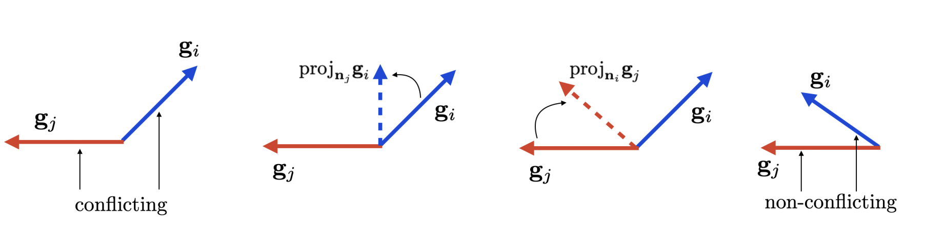
In multi-task learning we are interested in learning a policy for multiple tasks using a single network. However, most often the gradients of samples from different tasks conflict with the gradients of other tasks. One of the way to reduce such interferences is using gradient surgery. The idea is to take the gradients of conflicting tasks and project them onto the normal vector of the other gradient. This way we remove the opposing vectors of the gradients between tasks.

Scaling laws for Batch Size

The optimal batch size during training changes. Gradient-Norm Scale (GNS) acts as good proxy for guiding the selection of batch size (Gray et al., 2024). And per-sample gradient norms are essential for calculating GNS. Although we don’t need to instantiate per-sample gradients for this thanks to a clever trick which I will explain at the end, but still per-sample gradients can be a helpful tool to realize this.

Differential Privacy

Differential Privacy (DP) aims to protect individual privacy by adding noise to the gradients during training, preventing the model from memorizing specific training examples. The core mechanism involves computing per-sample gradients for each training example and clipping them to bound their influence, followed by adding calibrated noise to the aggregated gradients. The noise scale is determined by the desired privacy budget $(\epsilon, \delta)$ and the sensitivity of the computations, which is controlled through gradient clipping. This technique ensures that the presence or absence of any single training example has a limited impact on the model’s learned parameters, making it difficult to extract individual information from the trained model.

Per-sample Gradients for Transformers

There are many great blogs that explain the working of transformers, so I will just explain the components of the transformer that we need to consider for per-sample gradients calculations. Then we are going to go through each one of them and see how they can be converted towards per-sample gradients.

The main layers of the transformer that we need to consider to develop per-sample gradients are 1) Multi-Layer Perceptron 2) Self-Attention 3) Embeddings.

Linear Layer Let’s start with understanding the linear layer, as it forms the fundamental building block for more complex neural network architectures. A linear layer performs the transformation $y = Wx + b$, where $W$ is the weight matrix, $x$ is the input vector, and $b$ is the bias term. When processing a batch of samples, this becomes: \(Y = WX + b\) where $X$ is now a matrix with each column representing a sample in our batch. The key insight for computing per-sample gradients is understanding how the loss for a single sample $i$ relates to the parameters $W$ and $b$.

For a single sample, the gradient of the loss $L_i$ with respect to the weight matrix $W$ can be computed using the chain rule:

This expands to:

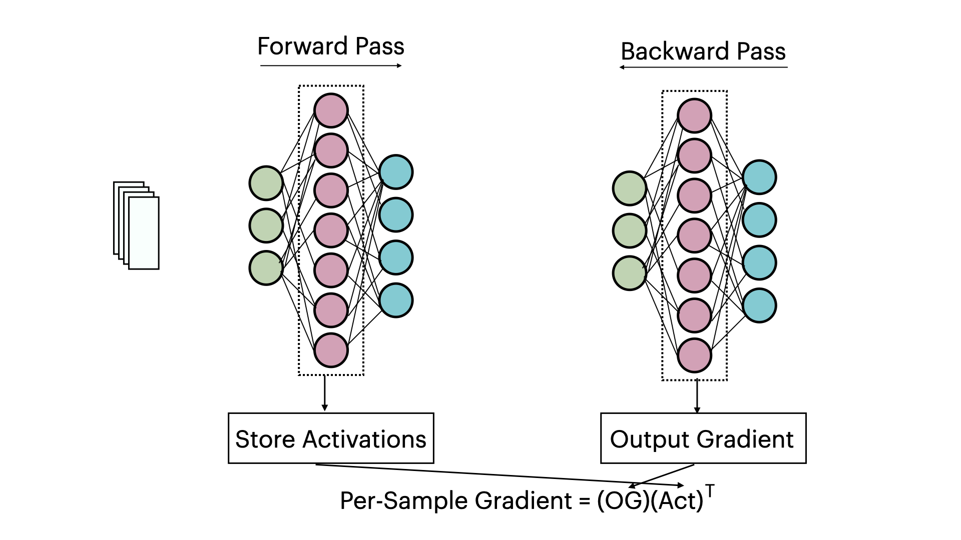
where $\frac{\partial L_i}{\partial y_i}$ is the gradient of the loss with respect to the layer’s output (which we receive during backpropagation from backward hook) and $x_i^T$ is the transposed input vector for sample $i$. This outer product gives us the per-sample gradient for the weights.

Multi-Layer Perceptron (MLP)

Let’s start with understanding how an MLP layer works in a transformer. At its core, an MLP consists of linear transformations with non-linear activations between them. For simplicity, let’s consider a single MLP layer:

where $W$ is the weight matrix, $x$ is the input vector, $b$ is the bias term, and $\sigma$ is a non-linear activation function (typically GELU in modern transformers).

To compute per-sample gradients for an MLP layer, we need to calculate $\frac{\partial L_i}{\partial W}$ and $\frac{\partial L_i}{\partial b}$ for each sample $i$. Using the chain rule:

Breaking this down:

• $\frac{\partial L_i}{\partial z_i}$ is the gradient of the loss with respect to the activation output
• $\frac{\partial z_i}{\partial y_i} = \sigma’(y_i)$ is the derivative of the activation function
• $\frac{\partial y_i}{\partial W} = x_i^T$ as we saw in the linear layer case

Therefore, the complete per-sample gradients for an MLP layer are:

\(\nabla W_i = \left(\frac{\partial L_i}{\partial z_i} \sigma'(y_i)\right) x_i^T\) \(\nabla b_i = \frac{\partial L_i}{\partial z_i} \sigma'(y_i)\)

In practice, transformers typically use two MLP layers with a GELU activation in between:

The per-sample gradients for this two-layer MLP can be computed by applying the chain rule repeatedly through both layers. This computation can be done efficiently by maintaining intermediate activations during the forward pass and reusing them during the backward pass.

Self-Attention Mechanism

Let’s now examine how to compute per-sample gradients for the self-attention mechanism, which is another crucial component of transformers. The self-attention mechanism can be broken down into several steps, each requiring careful consideration for per-sample gradient computation.

The self-attention operation can be expressed as:

where Q, K, and V are obtained through linear transformations of the input x:

To compute per-sample gradients, we need to calculate the gradients with respect to the weight matrices $W_q$, $W_k$, and $W_v$ for each sample. Let’s break this down step by step.

1. Query, Key, and Value Transformations For each sample i, we first need to compute the gradients for the linear transformations:

2. Attention Scores The attention scores computation involves a matrix multiplication followed by scaling:

The gradient through this operation needs to account for both the scaling factor and the matrix multiplication:

3. Softmax Operation Let $A_i = \text{softmax}(S_i)$ be the attention weights. The gradient through the softmax operation for sample i is:

where $\odot$ represents element-wise multiplication.

4. Final Output The final attention output for sample i is:

The gradients with respect to the attention weights and values are:

Efficient Implementation

To efficiently compute these per-sample gradients, we can use the einsum operation similar to the linear layer case. For example, the gradient computation for $W_q$ can be implemented as:

def compute_query_grad_sample(self, activations, grad_output):
    """
    Compute per-sample gradients for query projection matrix
    """
    return torch.einsum('b...n,b...m->b...nm', grad_output, activations)

The complete per-sample gradients for the attention mechanism are:

where each gradient component is computed using the chain rule through the attention operations described above.

Multi-Head Attention

For multi-head attention, we simply need to apply these computations independently for each attention head. The per-sample gradients for each head can be computed separately and then concatenated appropriately. If we have h heads, each with dimension d_h, the weight matrices are shaped accordingly:

• $W_q \in \mathbb{R}^{h \times d_{model} \times d_h}$
• $W_k \in \mathbb{R}^{h \times d_{model} \times d_h}$
• $W_v \in \mathbb{R}^{h \times d_{model} \times d_h}$

The final output projection matrix $W_o \in \mathbb{R}^{d_{model} \times hd_h}$ combines the outputs from all heads, and its per-sample gradients can be computed similarly to a standard linear layer.

Embeddings

The embedding layer, while seemingly different from linear layers, can actually be viewed as a special case of a linear transformation. Let’s understand how we can compute per-sample gradients for embeddings efficiently.

For an embedding layer with vocabulary size $V$ and embedding dimension $d$, we have an embedding matrix:

The embedding lookup operation for a token index $i$ can be expressed as multiplication with a one-hot vector $x \in {0,1}^V$:

where $x$ has a 1 in the $i$-th position and 0 elsewhere.

The key insight for computing per-sample gradients is that due to the one-hot nature of the input, the gradient computation becomes very sparse. For a single token, the gradient with respect to the embedding matrix is only non-zero at the row corresponding to that token:

where $\otimes$ represents the outer product and $\frac{\partial L_i}{\partial h}$ is the gradient with respect to the embedding output.

For a sequence of tokens in a single sample, we simply accumulate these gradients:

where $T$ is the sequence length, and $i$ denotes the sample index.

This computation is particularly efficient because we only need to update the rows of the gradient matrix corresponding to the actual tokens in our sequence, rather than performing full matrix operations. The sparsity of the input (one-hot vectors) means we can directly index and accumulate gradients at the relevant positions.